SOEN Architecture
Understanding the structure and components of Superconducting Optoelectronic Networks
SOEN Architecture Overview
The Superconducting Optoelectronic Network (SOEN) framework implements structured neural networks using differential equations that model physical superconducting devices. The architecture is built around layers connected by weighted connections, all governed by a simulation configuration.
Core Components
1. SOENModelCore
The central orchestrator that:
- Manages layer collection and connections
- Handles forward propagation through time
- Enforces parameter constraints
- Tracks network state and history
2. Layer System
Modular components implementing specific dynamics, from physical device models to virtual neural network layers.
3. Connection Framework
Flexible inter-layer connectivity with masks, constraints, and connection types.
4. Simulation Engine
Configurable time-stepping with multiple solver options and noise modeling.
Example Network Architecture
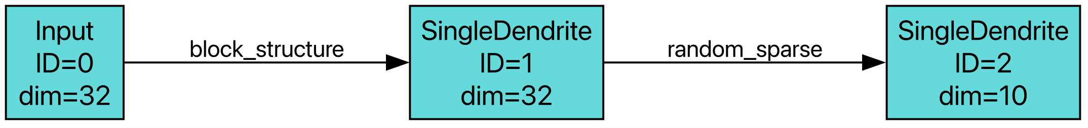
Example SOEN network showing layer connectivity and information flow
Layer Types
SOEN provides two categories of layers: Physical SOEN layers that model superconducting devices, and Virtual layers that implement standard neural network components.
Physical SOEN Layers
SingleDendriteLayer
Models a single-compartment superconducting device with dynamics:
ds/dt = γ₊ × g(φ) - γ₋ × sKey Parameters:
γ₊, γ₋(gamma_plus/minus): Coupling strengthsg(φ): Source function (e.g., tanh, zero-inductance)φ: External flux from upstream connectionss: Internal state variable
Features:
- Optional internal connectivity (
internal_J) - Multiple solver support (Forward Euler, Adaptive ODE, Parallel Scan)
- Power tracking for physical analysis
- Constraint enforcement
Physical Meaning: Represents a single Josephson junction or superconducting loop with flux-dependent dynamics.
DoubleDendrite1Layer & DoubleDendrite2Layer
Extended multi-compartment models with richer dynamics for more complex superconducting structures.
ScalingLayer
Provides parameter scaling and normalization for physical units and dimensionless quantities.
Virtual Layers
Standard Recurrent Layers
- RNNLayer: Basic recurrent neural network
- LSTMLayer: Long Short-Term Memory with gates
- GRULayer: Gated Recurrent Unit
- MinGRULayer: Minimal GRU implementation
- LeakyRNNLayer: RNN with leaky integration
Specialized Layers
- InputLayer: Data input and preprocessing
- ClassifierLayer: Output classification with optional batch normalization
Layer Base Class
All layers inherit from SOENBaseLayer which provides:
// Core attributes
dim: number              // Layer dimensionality
dt: number              // Time step
source_function         // Physics-based activation
track_power: boolean    // Power consumption tracking
physical_units: boolean // Physical vs dimensionless units

// Physical constants
PHI0 = 2.067833848e-15  // Flux quantum
Ic = 100e-6            // Critical current
wc = 7.79e11          // Characteristic frequency
Connection System
SOEN uses a sophisticated connection system that supports various connectivity patterns between layers.
Connection Types
External Connections
Connect different layers with the constraint: to_layer > from_layer (forward-only)
// Example connection config
ConnectionConfig({
    from_layer: 0,
    to_layer: 2,
    connection_type: "dense",
    params: {init_scale: 0.1}
})
Internal Connections
Self-connections within a layer (recurrent dynamics)
// Internal connectivity
ConnectionConfig({
    from_layer: 1,
    to_layer: 1,  // Same layer
    connection_type: "sparse",
    params: {sparsity: 0.1}
})
Connection Building
The build_weight function creates connection matrices with:
- Weight Matrix: Learnable parameters
- Connection Mask: Fixed connectivity pattern
- Constraints: Parameter bounds and structure
Connection Constraints
Connections can enforce various constraints:
- Sparsity patterns: Fixed zero elements
- Symmetry: Symmetric weight matrices
- Sign constraints: Positive/negative weights
- Magnitude bounds: Parameter ranges
Simulation & Solvers
SOEN supports multiple numerical integration methods for the differential equations.
Solver Types
Forward Euler (FE)
Simple explicit integration:
s(t+dt) = s(t) + dt × ds/dt
Pros: Fast, stable for small dt Cons: First-order accuracy Best for: Quick prototyping, real-time applications
Adaptive ODE (torchdiffeq)
High-precision adaptive integration using PyTorch's torchdiffeq
Pros: High accuracy, adaptive step size Cons: Computational overhead Best for: Research, high-precision simulations
Parallel Scan (PS)
Efficient parallel computation for linear systems
Pros: Highly parallelizable, GPU-optimized Cons: Limited to specific dynamics (no internal connectivity, state-independent source functions) Best for: Large-scale simulations without recurrence
Solver Selection Logic
The framework automatically handles solver compatibility:
- Internal connections → Fallback to Forward Euler
- State-dependent source functions → No Parallel Scan
- Default: Forward Euler for reliability
Noise & Perturbations
Stochastic Noise
Applied at each timestep to physical parameters:
NoiseConfig({
    phi: 0.01,           // Phase noise
    g: 0.005,           // Conductance noise
    s: 0.0,             // State noise
    bias_current: 0.002, // Bias current noise
    j: 0.0,             // Josephson coupling noise
    relative: true       // Relative vs absolute noise
})
Deterministic Perturbations
Fixed offsets with optional Gaussian spread:
PerturbationConfig({
    phi_mean: 0.1,      // Mean offset
    phi_std: 0.02,      // Standard deviation
    // ... similar for other parameters
})
Model Execution Flow
Forward Pass
Initialization
- Set initial states for all layers
- Apply noise/perturbation settings
- Initialize connection weights
Time Integration Loop
for t in range(time_steps):
    # Compute inter-layer fluxes
    phi_inputs = compute_connections(layer_states)

    # Update each layer
    for layer in layers:
        layer_states[layer] = layer.forward(
            phi_input=phi_inputs[layer],
            dt=self.dt
        )

    # Track history and power
    if tracking_enabled:
        update_histories()
Output Processing
- Extract final states or time series
- Apply time pooling (max, mean, final, etc.)
- Generate predictions
Configuration-Driven Design
Models are built entirely from YAML configuration:
# Example model specification
layers:
  - layer_id: 0
    layer_type: "Input"
    params: {dim: 10}

  - layer_id: 1
    layer_type: "SingleDendrite"
    params: {dim: 20, solver: "FE"}

  - layer_id: 2
    layer_type: "Classifier"
    params: {dim: 5}

connections:
  - from_layer: 0
    to_layer: 1
    connection_type: "dense"

  - from_layer: 1
    to_layer: 2
    connection_type: "sparse"
    params: {sparsity: 0.1}
This enables rapid experimentation and systematic architecture search.
Architecture Visualization
Interactive architecture diagrams coming soon
Will show layer connectivity and data flow patterns